
Volume
6, Number 2, Spring 2006
Development of a Cost Model
for Manual Tool Polishing
|
Kenneth J. Fisher |
Michael J. Lobaugh |
|
School of Engineering & Engineering
Technology |
School of Engineering & Engineering
Technology |
|
|
|
|
Robert M. Michael |
Shannon K. Sweeney |
|
School of Engineering & Engineering
Technology |
School of Engineering & Engineering
Technology |
|
|
|
|
Peter J. Kuvshinikov |
|
Tool & Die Productions |
|
|
ABSTRACT
This paper describes the development of a cost analysis model using a knowledge-based approach that allows a prediction of the total time required to complete a manual polishing operation. Parameters considered within the model include the impact upon polishing time caused by total surface finishing area, polish surface geometry and complexity, final surface finish requirements, part weight, part quantity, substrate material, and required finish tolerances.
The cost model evaluates the impact of each factor by assigning weights and values based upon shop level process knowledge acquired during nearly twenty years of experience in manual finishing operations of production parts. To validate the model, predicted polishing times from the cost model are compared to actual costs resulting from the production of a controlled sample of parts. Recommendations for continuance of the study are made to expand the model’s accuracy, range and utility.
INTRODUCTION
In the machining and tooling industry, secondary manual polishing is almost always required after initial tool fabrication has been completed. The extent of polishing can range from simply deburring the tool in a production shop, to developing a high optical finish of cavity and core surfaces as typically found in injection molds normally completed in a specialty polishing shop.
Manual polishing is the hand finishing of various metal surfaces using abrasive materials to improve the quality of the finish and required precision tolerance of a work surface. Considering the often-required application of manual polishing and the long history of its use, it is surprising that little information in the literature exists relating to the subject of hand finishing. Hand finishing of tool components has always been a trained skill that was developed over a lifetime. Since there is a trend toward specialization of toolmakers in expanding fields of machining, fewer toolmakers are being trained to be proficient in manual polishing and the process of hand finishing is slowly disappearing from the toolmaker’s knowledge base.
The literature cites the development of cost estimation methods influenced by design and process parameters for a variety of manufacturing processes. Much of the most recent efforts have been directed at providing design engineers with means to select a suitable manufacturing process early in the design configuration stage during Design for Manufacture (DFM). Integrated within this work is the formulation of guidelines allowing the designer to either reconfigure the concept model to lower the cost or to design for alternate, lower cost manufacturing processes. Examples include the prediction of relative tooling and part costs for injection molding using dimensions, locations, and orientation of features to evaluate part manufacturability and cost as described by Poli 1 or the prediction of the fabrication time required for the production of components by a variety of process types based on part features and manufacturing parameters as outlined by Boothroyd, Dewhurst, and Knight 2. Research by Swift and Booker 3, and by Ashby 4 provides design information in terms of charts or computer programs to guide design for process and early cost estimation during initial product development. Unfortunately, little similarly related research has been conducted allowing the prediction of processing time and costs associated with manual polishing as driven by design and process parameters.
Research in the field of surface polishing has largely been directed toward automated rather than manual tool finishing. Much of the automated polishing research has been directed at computer controlled (robotic) mold finishing typically like that described by Lui 5 or at areas such as ultrasonic flow polishing as outlined by Jones 6 describing alternatives to time consuming manual methods. However, a substantial number of molds continue to be finished by manual polishing while awaiting the continued development and wide scale adoption of these newer methods.
The research most directly related to manual polishing has been directed toward the development of improved abrasives and ultrasonic abrasive hand tools. Published literature related to the time required for manual polishing is almost non-existent other than several basic guidelines as described in handbooks. Today there are no known models for predicting the time and cost required to perform a manual polishing operation nor is there data which defines the design and process parameters that drive these costs. Superficial data does exists as described by Rosato 7 stating that polishing can represent 5-30% of the mold cost and that costs can vary linearly from no additional secondary finishing cost for a 30 micro inch (0.76 micron) surface finish to $4.00 per square inch for a 5 micro inch (0.127 micron) surface finish. Therefore, the goal of this paper is to define the design and process parameters that influence the cost of manual polishing. The information derived by this study can be used to establish cost and design guidelines for design engineers and provide a system for consistent cost estimation for those involved in the quotation of manually polished parts.
DEVELOPMENT OF THE COST MODEL
The development of the model is based upon shop level process knowledge as defined by Chang 8. The process knowledge used is based on nearly twenty years of shop experience for manual polishing, covering a wide variety of part configurations and surface conditions.
To limit variability in the study from bias associated with preferential customer treatment or by cost adjustments made for the purposes of competitive bidding, a single customer was selected for the comparison of predicted to actual results. The selected customer had an established history of repeated orders, was a major contributor to total shop orders placed, placed orders in varying lots sizes ranging from small to large, and required finish operations covering the majority of the attributes attempted by the cost model. The model’s construct follows closely the costing model formulated by Swift 3 while creating customer specification and process driven cost coefficients that allow a comparison of any given polish operation to an ideal polishing situation.
A spectrum of candidate polished parts was evaluated to determine the major characteristics that distinguish each part from the rest of the candidates. This review resulted in the identification of seven key characteristics. The polishing surface area, final surface finish requirements, and complexity of the surface area to be polished are driven by customer specifications. The part weight, quantity of parts, substrate material, and number of critical tolerances to be held are key design factors that influence the processing of the polished components, and mandate the methods employed by the polisher. Following the method of Swift, predicted total polishing time in hours, PT, was formulated as:
PT = CS * PD (1)
Where:
CS = Customer specification factors
PD = Process driven factors
DESCRIPTION OF PRIMARY
COEFFICIENTS
The customer specifications dictate the first three primary coefficients involving the amount of surface area to be polished, the geometric complexity of the area to be polished, and the final required surface finish. The customer specification factors thus determine the geometric constraints and, given the initial degree of finish of the substrate, the number of polishing operations. Using the approach of Swift, these relations are linked as:
CS = AC * GC * FC (2)
Where:
AC = Area coefficient
GC = Geometric complexity coefficient
FC = Surface finish coefficient
The part weight, material characteristics of the polishing surface, the required tolerances of the finished surface and the quantity of similar parts ordered are the process driven factors. The process driven factors dictate the methods by which the parts are to be polished, and they will have an effect on the time and handling of the parts.
PD = WC * QC * MC * TC (3)
Where:
WC = Weight coefficient
QC = Batch quantity coefficient
MC = Substrate material coefficient
TC = Tolerance coefficient
The cost model is based on the combination of customer specification factors and process driven factors allowing a prediction of total polishing cost, PC, formulated as:
PC = PT * M (4)
Where:
PT = Predicted total polishing time, hours
M = Operator rate
DEVELOPMENT OF COEFFICIENTS
Each coefficient value was developed utilizing shop level knowledge-based information. A base line, ideal condition with all of the coefficients equaling one would result in a single hour to polish one square inch of an electric discharge machine (EDM) substrate surface to a 400-grit paper finish. As the coefficient increases or decreases there is a weighted corresponding increase or decrease in the time required to complete the polishing operation.
AREA COEFFICIENT
This area coefficient, Figure1, was developed from knowledge gained from the experience of polishing a wide range of surface areas. It was determined that there was not a direct linear correlation between area size and time to complete the required finish. The minimum base factor of one is determined by the typical time required to polish one square inch of EDM produced surface area to a 400-grit paper finish.
The variation from the baseline is primarily due to the fact that initial setup time has already been invested with the first square inch of polishing area. Every additional square inch of area added to the polishing surface will increase time and cost. After the first several square inches have been polished, the curve reflects less of an increase as the surface area further expands. This is because in the process of polishing, a greater percentage of time is required to carefully and consistently polish around the edges or borders of a surface. As the surface area increases, the perimeter or border grows at a much slower rate and thus the ratio of surface to perimeter decreases. For example, a one square inch surface area has four linear inches of perimeter (1:4) while a 16 square inch area has 16 linear inches of perimeter (1:1). The area curve stops at 20 square inches due to limited available shop knowledge in this range.
PART COMPLEXITY COEFFICIENT
The part complexity coefficient, Figure 2, is based on a relationship between the accessibility to a polishing surface and the degree of geometric complexity the surface contains. An easily accessible area and a simple or concentric geometry will have a low number as a multiplier and a part with very limited accessibility and complex geometry will have a higher value. Symmetrical part geometry characteristics are reflected in those parts that can be spun polished along a single uniform axis. Non-symmetrical parts are polish surfaces that do not lend themselves to the ability to be spun. External or open geometry characteristics are those where the polishing area is fully accessible in several orientations. Conversely, internal geometry characteristics are those where the polishing area is within a cavity with limited accessibility. Shallow ribs are defined as having a depth to width ratio of no more than three to one and greater ratios are defined as deep ribs.
|
|
Figure 2 - Part Complexity Value (GC) |
|
||||
|
|
|
|
||||
|
|
Part Geometry |
|
|
|||
|
|
|
|
|
|||
|
Polishing |
Symmetrical |
Non-Symmetrical |
Non-Symmetrical |
Non-Symmetrical |
||
|
Area |
(spin polish) |
(flats and curves) |
(fine ribs) |
(deep ribs) |
||
|
|
1E (Coefficient 0.4) |
2E
(Coefficient 0.65) |
3E
(Coefficient 1.6) |
4E
(Coefficient 2.7) |
||
|
Simple external geometry or easily assessable internal areas with 1:1 ratio depth to width |
|
|
|
|
||
|
|
|
|
|
|
||
|
|
1M
(Coefficient 0.5) |
2M
(Coefficient 1.4) |
3M
(Coefficient 2.3) |
4M
(Coefficient 3.7) |
||
|
Semi-complex external geometry or moderately assessable to internal areas with 1-3:1 ratio depth to width |
|
|
|
|
||
|
|
1L
(Coefficient 0.9) |
2L (Coefficient 2.2) |
3L
(Coefficient 2.8) |
4L
(Coefficient 5.0) |
||
|
Complex external geometry or limited accessibility to
internal areas with 3+:1 ration depth to width |
|
|
|
|
||
|
|
|
|
|
|
||
|
|
|
|
|
|
||
|
Note: The area in
blue represents the internal area to be polished. |
|
|
||||
|
|
|
|
||||


FINISH VALUE COEFFICIENT
The finish value is a relationship between the initial finish (machined surface) and the required final finish. The coefficient, as shown in Figure 3, is based on three primary machining surfaces being manually polished to one of twelve SPI/SPE finished surface requirements. The coefficient values have the lowest values at the upper left corner of the chart with a fine start finish and a coarse polished finish. As the start finish becomes coarse and/or the polish finish becomes finer the coefficient value will increase. An example of this is that it would take one hour to polish one square inch of an EDM finish to a B2 (400 paper) finish, likewise it would require two hours to polish one square inch of an EDM finish to an A3 (15 diamond) finish.
|
|
|
Figure 3 – Surface Finish Coefficient (FC) |
|
|
|||||
|
|
|
|
|
|
|||||
|
|
SPI Mold Finish Index |
||||||||
|
Start |
|
|
|
|
|
|
|
|
|
|
Finish |
C3 / D3* |
C2 / D2* |
C1 / D1* |
B3 |
B2 |
B1 |
A3 |
A2 |
A1 |
|
|
320 stone |
400 stone |
600 stone |
320 grit paper |
400 grit paper |
600 grit paper |
15 diamond |
6 diamond |
3 diamond |
|
|
|
|
|
|
|
|
|
|
|
|
Fine |
|
|
|
|
|
|
|
|
|
|
Finish |
(coeff. 0.2) |
(coeff. 0.3) |
(coeff. 0.4) |
(coeff. 0.6) |
(coeff. 0.8) |
(coeff. 1.0) |
(coeff. 1.4) |
(coeff. 2.0) |
(coeff. 3.5) |
|
(ground) |
|
|
|
|
|
|
|
|
|
|
|
|
|
|
|
|
|
|
|
|
|
Medium |
|
|
|
|
|
|
|
|
|
|
Finish |
(coeff. 0.4) |
(coeff. 0.5) |
(coeff. 0.6) |
(coeff. 0.8) |
(coeff. 1.0) |
(coeff. 1.2) |
(coeff. 2.0) |
(coeff. 2.5) |
(coeff. 4.0) |
|
(EDM) |
|
|
|
|
|
|
|
|
|
|
|
|
|
|
|
|
|
|
|
|
|
Coarse |
|
|
|
|
|
|
|
|
|
|
Finish |
(coeff. 0.8) |
(coeff. 0.9) |
(coeff. 1.1) |
(coeff. 1.5) |
(coeff. 1.8) |
(coeff. 2.0) |
(coeff. 2.6) |
(coeff. 3.0) |
(coeff. 4.5) |
|
(milled) |
|
|
|
|
|
|
|
|
|
|
|
|
|
|
|
|
|
|
|
|
|
*Note: same finish
required prior to dry blast |
|
|
|
|
|
|
|||
|
|
|
|
|
|
|
|
|||
|
|
|
Figure 4 - Part Polishing Steps |
|
|||||||
|
Polishing Steps |
|
|
|
|
|
|
|
|
|
|
|
(Stepping
up from finish to finish) |
|
|
|
|
|
|
|
|
||
|
|
|
|
|
|
|
|
|
|
|
|
|
A-1 #3 Diamond |
13 |
12 |
11 |
10 |
8 |
7 |
6 |
4 |
2 |
0 |
|
A-2 #6 Diamond |
11 |
10 |
9 |
8 |
6 |
5 |
4 |
2 |
0 |
2 |
|
A-3 #15 Diamond |
9 |
8 |
7 |
6 |
4 |
3 |
2 |
0 |
2 |
4 |
|
B-1 600 Paper |
7 |
6 |
5 |
4 |
2 |
1 |
0 |
2 |
4 |
6 |
|
B-2 400 Paper |
6 |
5 |
4 |
3 |
1 |
0 |
1 |
3 |
5 |
7 |
|
B-3 320 Paper |
5 |
4 |
3 |
2 |
0 |
1 |
2 |
4 |
6 |
8 |
|
C1/D1* 600 Stone |
3 |
2 |
1 |
0 |
2 |
3 |
4 |
6 |
8 |
10 |
|
C2/D2* 400 Stone |
2 |
1 |
0 |
1 |
3 |
4 |
5 |
7 |
9 |
11 |
|
C3/D3* 320 Stone |
1 |
0 |
1 |
2 |
4 |
5 |
6 |
8 |
10 |
12 |
|
EDM Surface |
0 |
1 |
2 |
3 |
5 |
6 |
7 |
9 |
11 |
13 |
|
|
EDM |
C3/D3* |
C2/D2* |
C1/D1* |
B3 |
B2 |
B1 |
A3 |
A2 |
A1 |
|
|
Surface |
320
stone |
400
stone |
600
stone |
320
paper |
400
paper |
600
paper |
#15
diamond |
#6
diamond |
#3
diamond |
|
|
|
|
|
|
|
|
|
|
|
|
|
|
|
|
|
|
Polishing Steps |
|
|
|
|
|
|
*Note: same finish required prior
to dry blast |
|
(Stepping up from finish to finish) |
|
|
|
|||||
|
EDM start finish is
used because it reflects 90% of all work evaluated in the model |
|
|
|
|||||||
The process driven factors are based on the number of steps required to complete a polished finish as shown in Figure 4. In the process of manual tool polishing the improvement of the surface finish is based on increasing the abrasive grit of the polishing agent. Between each of the finishes, time is required to remove the previous abrasive and prepare the polishing surface and surrounding area for the next finer abrasive. This is to eliminate contamination of the next finish surface. The polishing step chart is referenced to identify the number of finishing steps involved to reach a final polish and is used to determine the part weight and batch quantity coefficient.
PART WEIGHT
COEFFICIENT
This coefficient, shown in Figure 5, is based on the weight of each of the components. During the manual finishing process, the polishing surfaces often need to be reoriented to facilitate greater accessibility to a complex geometry. As the number of polishing operations increases, the heavier components require additional time for positioning and securing. The three groupings of polishing steps are simply broken down to a high, medium, and low number of steps. The weight classification is determined by the ease of handling each weight. Low weight parts can be easily maneuvered with one hand while medium weight parts require two hands to be maneuvered. High weight parts require mechanical assistance for safe handling.
|
Figure 5 - Part Weight Coefficient (WC) |
||||
|
Polishing
Steps |
|
|
|
|
|
(Finishing grades) |
|
|
|
|
|
|
|
|
|
|
|
High |
(coefficient 1.0) |
(coefficient 1.2) |
(coefficient 1.5) |
|
|
(over 9 steps) |
|
|
|
|
|
|
|
|
|
|
|
Medium |
(coefficient 1.0) |
(coefficient 1.15) |
(coefficient 1.4) |
|
|
(4 to 8 steps) |
|
|
|
|
|
|
|
|
|
|
|
Low |
(coefficient 1.0) |
(coefficient 1.1) |
(coefficient 1.3) |
|
|
(under 3 steps) |
|
|
|
|
|
|
|
|
|
|
|
|
Low (1-5 lb.) |
Medium (6-45 lb.) |
High (over 46 lb.) |
|
|
|
|
|
|
|
|
|
|
Weight of parts |
|
|
BATCH QUANTITY COEFFICIENT
The part quantity coefficient, Figure 6, is based on the fact that as the number of similar parts polished in each batch increases, the piece part cost reduction becomes more pronounced. This is primarily due to operator proficiency increase since operations are being repeated. Likewise if a large batch of similar parts requires a high number of operations to complete the required finish, the piece part cost will be reduced since a greater number of parts are finished together between subsequent polishing steps.
|
|
Figure 6 - Batch Quantity Coefficient (QC) |
||
|
Polishing
Steps |
|
|
|
|
(Stepping up from finish to finish) |
|
|
|
|
|
|
|
|
|
High |
(coefficient 1.1) |
(coefficient 0.9) |
(coefficient 0.7) |
|
(Over 9 steps) |
|
|
|
|
|
|
|
|
|
|
|
|
|
|
Medium |
(coefficient 1.2) |
(coefficient 1.0) |
(coefficient 0.9) |
|
(From 4 to 8 steps) |
|
|
|
|
|
|
|
|
|
|
|
|
|
|
Low |
(coefficient 1.3) |
(coefficient 1.1) |
(coefficient 1.1) |
|
(Under 3 steps) |
|
|
|
|
|
|
|
|
|
|
Low (1-10) |
Medium (11-51) |
High (above 51) |
|
|
|
|
|
|
|
|
Part Quantity |
|
SUBSTRATE MATERIAL
COEFFICIENT
The material coefficient is primarily based on the relationship between the surface hardness of the tool to be polished and the initial condition of the substrate surface prior to finishing as shown in Figure 7. A higher coefficient value is added if coarse tool marks need to be removed from a hard material rather than fine grind marks from a soft material.
|
|
Figure 7 - Substrate Material Coefficient (MC) |
||
|
Start
Finish |
|
|
|
|
|
|
|
|
|
Coarse |
(coefficient 0.85) |
(coefficient 1.2) |
(coefficient 3.0) |
|
(milled) |
|
|
|
|
|
|
|
|
|
Medium |
(coefficient 0.82) |
(coefficient 1.0) |
(coefficient 1.8) |
|
(EDM) |
|
|
|
|
|
|
|
|
|
Fine |
(coefficient 0.8) |
(coefficient 0.9) |
(coefficient 1.6) |
|
(ground) |
|
|
|
|
|
Soft (below 60 Rb) |
Medium (60 Rb - 58 Rc) |
High (above 58 Rc) |
|
|
Aluminum, BeCu |
H-13, 420 SS |
Carbide |
|
|
|
|
|
|
|
|
Material Hardness |
|
TOLERANCE VALUE COEFFICIENT
The polishing of highly critical dimensioned parts requires additional time to carefully and consistently remove material stock from the polished surface, Figure 8. On high tolerance surfaces the amount of stock removed in each step has to be measured and sometimes documented. The tolerance value coefficient takes into consideration the fact that as the areas of critical dimensions increase from one to three datums the coefficient value will increase. The base line of the factor of 1 is based on the most common tolerance condition.
|
|
Figure 8 - Tolerance Coefficient (TC) |
||
|
|
|
|
|
|
Critical Dimension |
|
|
|
|
|
|
|
|
|
Across 3 datums |
(coefficient 0.85) |
(coefficient 1.3) |
(coefficient 2.0) |
|
|
|
|
|
|
|
|
|
|
|
Across 2 datums |
(coefficient 0.8) |
(coefficient 1.2) |
(coefficient 1.75) |
|
|
|
|
|
|
|
|
|
|
|
Across 1 datum |
(coefficient 0.8) |
(coefficient 1.0) |
(coefficient 1.6) |
|
|
|
|
|
|
|
Low (0.01") |
Medium (0.001") |
High (0.0005") |
|
|
|
|
|
|
|
Required Tolerance Specifications |
||
|
|
|||
EXAMPLE OF MODEL USE
|
Table 1 Sample Part Data - Polishing Analysis Model |
||||||||||||
|
Component Details |
CS = AC *
GC * FC |
|
PD = WC *
QC * MC * TC |
PT = CS *
PD |
||||||||
|
Part |
Part(CV) |
Polished |
Complexity |
Finish |
Customer |
Part(WC) |
Part(QC) |
Material |
Tolerance |
Process |
Predicted |
Actual |
|
ID |
Shape |
Area (AC) |
Value (GC) |
(FC) |
Spec.(CS) |
Weight |
Quantity |
Value(MC) |
(TC) |
Driven(PD) |
Time(PT) |
Time(AT) |
|
1 |
3M |
2.0 |
2.3 |
2.0 |
9.2 |
1.0 |
0.7 |
1.0 |
1.0 |
0.7 |
6.44 |
6.75 |
MODEL VALIDATION
Data derived from 29 polishing orders from one customer was used to test the validity of the model. The selection of only one customer was done to eliminate any bias that may exist between customers. The selected customer’s work covers approximately 90% of all the jobs performed within the author’s facility and specifications were derived from part drawings and finish requirements provided by the customer. This data was evaluated and placed into the analysis charts, as shown in Table 2, to develop a predicted time frame to manually polish each part. After completing the analysis, the actual work records were pulled for each order and the actual time to produce the parts recorded in the table for comparison. Figure 9 shows the correlation between the actual and predicted times.
Although the model is not perfect, a correlation analysis shows that the time (or cost) model is statistically merited. The correlation coefficient r for the sample is 0.9518. A hypothesis test 9 shows that there is a correlation with virtual certainty. From the sample, the confidence interval 9 for the correlation coefficient of the population is 0.8988 to 0.9774 (95%, 2-sided). The coefficient of determination r2 for the sample is 0.9059. The coefficient of determination is defined as the explained variation divided by the total variation. The fact that more than 90% of the observed variation is explained is desirable.
The slope m for the sample is 0.8795. From the sample, the confidence interval 10 for the slope of the population is 0.7676 to 0.9914 (95%, 2-sided). The fact that this interval does not include unity is undesirable. However, note that the upper limit is quite close to unity. This result indicates that, on the average, the time model will underestimate the actual time. An underestimation of time may be viewed as undesirable to anyone using the tool for quoting purposes as it could adversely affect profits.
The intercept b for the sample is 0.1259. From the sample, the confidence interval 9 for the intercept of the population is -0.0127 to 0.2645 (95%, 2-sided). The fact that this interval includes zero is desirable. The prediction interval 10 is the range of statistically possible values of y (actual hours) for a given value of x (predicted hours). That is, for a predicted time of two hours for example, the actual time for individual part configurations is expected to be between about 1.4 and 2.4 hours, with 95% confidence.
|
Table 2 Validation Data - Polishing
Analysis Model |
||||||||||||
|
Component Details |
CS = AC *
GC * FC |
|
PD = WC *
QC * MC * TC |
PT = CS *
PD |
||||||||
|
Part |
Part(CV) |
Polished |
Complexity |
Finish |
Customer |
Part(WC) |
Part(QC) |
Material |
Tolerance |
Process |
Predicted |
Actual |
|
ID |
Shape |
Area (AC) |
Value (GC) |
(FC) |
Spec.(CS) |
Weight |
Quantity |
Value(MC) |
(TC) |
Driven(PD) |
Time(PT) |
Time(AT) |
|
1 |
1E |
1 |
0.4 |
0.4 |
0.16 |
1 |
1.1 |
0.9 |
1 |
0.99 |
0.1584 |
0.143 |
|
2 |
1E |
2.1 |
0.4 |
2 |
1.68 |
1 |
0.7 |
0.9 |
1 |
0.63 |
1.0584 |
1.1 |
|
3 |
1E |
2.2 |
0.4 |
2.5 |
2.2 |
1 |
0.9 |
1 |
1 |
0.9 |
1.98 |
1.92 |
|
4 |
1E |
4 |
0.4 |
0.4 |
0.64 |
1 |
1.3 |
1 |
1 |
1.3 |
0.832 |
0.643 |
|
5 |
1E |
1 |
0.4 |
0.4 |
0.16 |
1 |
1.1 |
0.9 |
1 |
0.99 |
0.1584 |
0.214 |
|
6 |
1E |
1 |
0.4 |
2 |
0.8 |
1 |
0.9 |
1 |
1 |
0.9 |
0.72 |
0.46 |
|
7 |
2E |
2.2 |
0.65 |
0.4 |
0.572 |
1 |
1.1 |
0.9 |
1 |
0.99 |
0.56628 |
0.571 |
|
8 |
2E |
1.4 |
0.65 |
0.4 |
0.364 |
1 |
1.1 |
0.9 |
1 |
0.99 |
0.36036 |
0.393 |
|
9 |
2E |
2 |
0.65 |
0.4 |
0.52 |
1 |
1.1 |
0.9 |
1 |
0.99 |
0.5148 |
0.464 |
|
10 |
2E |
3.6 |
0.65 |
0.4 |
0.936 |
1 |
1 |
0.9 |
1 |
0.9 |
0.8424 |
0.714 |
|
11 |
2E |
1.9 |
0.65 |
0.4 |
0.494 |
1 |
1.1 |
0.9 |
1 |
0.99 |
0.48906 |
0.518 |
|
12 |
2E |
1.8 |
0.65 |
1 |
1.17 |
1 |
0.9 |
0.9 |
1 |
0.81 |
0.9477 |
1.14 |
|
13 |
2E |
1.1 |
0.65 |
1 |
0.715 |
1 |
0.9 |
0.9 |
1 |
0.81 |
0.57915 |
0.518 |
|
14 |
2E |
5.6 |
0.65 |
0.4 |
1.456 |
1 |
1.3 |
0.9 |
1 |
1.17 |
1.70352 |
2.32 |
|
15 |
2E |
1.1 |
0.65 |
1 |
0.715 |
1 |
1.2 |
0.82 |
1 |
0.984 |
0.70356 |
1.06 |
|
16 |
3E |
1 |
1.6 |
1 |
1.6 |
1 |
1.2 |
1 |
1 |
1.2 |
1.92 |
1.78 |
|
17 |
3E |
1.7 |
1.6 |
1 |
2.72 |
1 |
0.9 |
0.9 |
1 |
0.81 |
2.2032 |
2.39 |
|
18 |
1M |
1.5 |
0.5 |
0.6 |
0.45 |
1 |
1.1 |
1 |
1 |
1.1 |
0.495 |
0.607 |
|
19 |
1M |
1 |
0.5 |
2 |
1 |
1 |
0.9 |
1 |
1 |
0.9 |
0.9 |
0.857 |
|
20 |
1M |
1 |
0.5 |
2 |
1 |
1 |
0.9 |
1 |
1 |
0.9 |
0.9 |
0.964 |
|
21 |
1M |
2 |
0.5 |
1.4 |
1.4 |
1 |
0.9 |
0.9 |
1 |
0.81 |
1.134 |
1.14 |
|
22 |
1M |
1 |
0.5 |
0.8 |
0.4 |
1 |
1.2 |
0.9 |
1 |
1.08 |
0.432 |
0.429 |
|
23 |
1M |
1 |
0.5 |
2 |
1 |
1 |
0.9 |
0.9 |
1 |
0.81 |
0.81 |
1.14 |
|
24 |
1M |
1.6 |
0.5 |
0.4 |
0.32 |
1 |
1.1 |
0.9 |
1 |
0.99 |
0.3168 |
0.357 |
|
25 |
2M |
1.25 |
1.4 |
0.3 |
0.525 |
1 |
1.1 |
0.9 |
1 |
0.99 |
0.51975 |
0.464 |
|
26 |
2M |
1 |
1.4 |
0.4 |
0.56 |
1 |
1.1 |
0.8 |
1 |
0.88 |
0.4928 |
0.607 |
|
27 |
2M |
1.4 |
1.4 |
0.4 |
0.784 |
1 |
1.1 |
0.9 |
1 |
0.99 |
0.77616 |
0.714 |
|
28 |
2M |
2.5 |
1.4 |
1.2 |
4.2 |
1 |
0.9 |
1 |
1 |
0.9 |
3.78 |
2.96 |
|
29 |
3M |
1 |
2.3 |
0.6 |
1.38 |
1 |
1.3 |
0.9 |
1 |
1.17 |
1.6146 |
1.61 |
MODEL UTILITY
Implementation of the model may improve the consistency in customer order quotation by eliminating customer bias, simplifying, and standardizing the bidding process within the manual polisher’s facility. This model provides a greater understanding on how jobs are processed and identifies the factors having the greatest impact on final cost. It also can be used to measure and evaluate the methods and procedures within the polisher’s facility (what works and what does not).
Tool design engineers can benefit from using the analysis model since it can identify design parameters that influence the cost of manual polishing. Information derived from the model could be used to judge the impact of an initial design and allow alteration of the design and construction of surfaces as needed to facilitate cost reductions at an early stage in the design process.
CONCLUSIONS AND
RECOMMENDATIONS
The cost model identifies seven cost drivers (coefficients) that determine the time required to complete a polishing operation. The value of each of the drivers was established against a baseline of one hour to polish one square inch of an EDM machined surface to a 400-paper finish. Statistical analysis reveals the model to have merit but that it tends to underestimate the actual time to complete the total polish operation.
Including operator rate, M, there are a total of eight factors (or main effects) that determine polishing cost, PC. Consequently there are 28 possible two-factor (low-order) interactions 56 possible three-factor interactions, and so on. A possible two-factor interaction between surface finish and tolerance is obvious because a small tolerance and a fine finish will usually not be independent contributors to polishing time. Other two-factor interactions may also exist.
The sparsity of effects principle 10 states that a system is usually dominated by the main effects and low-order interactions. Thus, three-factor and higher interactions are usually neglected. This work neglects high-order interactions and currently also neglects two-factor interactions. Evaluation of such interactions must be determined by shop level knowledge based information, similar to that done for main effects.
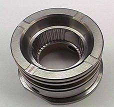
The greatest difficulty with the existing model is in determining the exact part complexity coefficient that needs to be assigned to the customer-specified factor. An example of this concern was present with the sample part. The part complexity coefficient reflects a part with an internal cavity that contains four shallow ribs. The sample part actually contains 36 ribs. The difference in the quantity of ribs reflects the lower estimated polishing time to the actual time required to polish the sample part. This is complicated further by the wide range of complex and unique shapes that need to be considered in determining a part complexity coefficient. In addition, the calculations are sensitive to the values derived from the area coefficient chart. Thus additional information needs to be developed for the coefficients related to part complexity and the polished surface area. Also, available information in these two areas needs to be expanded further to validate the model for parts with large surface areas and very complex geometry - particularly those in the range of 3-4L as described in Figure 2. Few parts within this range have been processed within the author’s shop and thus insufficient data exists to use in the validation of the model.
The knowledgebase model was developed from the author’s polishing shop experiences, skill level and performances. The developed chart coefficients may vary if this data is applied to other shop environments with different expertise and approaches.
The use of a computer software model would greatly enhance the model’s utility. A computerized model would allow the part complexity value chart to be expanded to cover a greater number of geometric changes in the complexity of a part to be polished. A software model would also remove any errors that may be produced with manual calculations and guide the user through the steps in applying the cost model.
Future development of the model awaits the continued bidding of future jobs at the author’s facility and then tracking the predicted time against the actual time required to complete the job. Hopefully, the knowledge gained from additional manual polishing orders will expand the range of geometric part diversity evaluated under the current model and allow further refinement and validation of the model’s accuracy and dependability. Additionally, the model should be applied at other polishing facilities to determine the impact of any bias resulting from this baseline study.
NOMENCLATURE
SPI Finish A-1 -- Grade #3, 6000 Grit Diamond Buff
SPI Finish A-2 -- Grade #6, 3000 Grit Diamond Buff
SPI Finish A-3 -- Grade #15, 1200 Grit Diamond Buff
SPI Finish B-1 -- 600 Grit Paper
SPI Finish B-2 -- 400 Grit Paper
SPI Finish B-3 -- 320 Grit Paper
SPI Finish C-1 -- 600 Grit Stone
SPI Finish C-2 -- 400 Grit Stone
SPI Finish C-3 -- 320 Grit Stone
SPI Finish D-1 -- 600 Stone Prior to Dry Blast Glass Bead #11
SPI Finish D-2 -- 400 Stone Prior to Dry Blast #240 Oxide
SPI Finish D-3 -- 320 Stone Prior to Dry Blast #24 Oxide
SPE -- The Society of Plastic Engineers
SPI -- The Society of the Plastic Industry
REFERENCES
[3] Swift, K., Booker, J., 1992, Process Selection from Design to Manufacture, 1st edition, Wiley & Sons, Inc., New York, NY, pp. 173-201.
[4] Ashby, M. 1992, Materials
Selection in Mechanical Design,
Pergamon Press,
[5] Lui, C., Tam, H., 1996, “To Speed Up Robotic Mold Polishing by Hand Tools,” Journal of Engineering and Applied Science, pp. 513-516.
[6] Jones, A.,
[7] Rosato, D., 1986, Injection Molding Handbook, Van Nostrand Reinhold Co., Inc., New York, NY, pp. 216-220.
[8] Chang, T., 1990, Expert
Process Planning for Manufacturing, Addison-Wesley,
[9] Spiegel, M., 1961, Theory and Problems of Statistics, Schaum’s Outline Series, McGraw-Hill
[10] Montgomery, D., Runger, G., 1999, Applied Statistics and Probability for Engineers, 2nd ed., John Wiley and Sons, Chap. 10